Analysis & Calculations

Every metric an audit reports is computed from the long-format dataset assembled in §08. This section defines each metric, works it through a single consistent example, and closes with the emissions layer — the companion dashboard that converts composition results into greenhouse-gas terms. Formulas are stated once, worked once, and accompanied by the mistakes each one invites.

The worked example

All calculations on this page use one dataset: a facility audit ("Maple Centre", spring event) that sampled all three streams over a five-day generation period with 120 employees on site. Stream totals: garbage 380 kg (five sorting samples), recycling 120 kg, organics 60 kg — 560 kg in all. Within the garbage stream: 130 kg food waste, 95 kg program-recyclable materials, and 155 kg residual. The recycling stream contained 14 kg of non-target material; the organics stream, 6 kg.

Composition

The distinction matters whenever samples differ in size, which is always. Two samples make the point: sample A is 100 kg with 30 kg food (30%); sample B is 20 kg with 2 kg food (10%). The average of the percentages is 20%; the true aggregate is 32 ÷ 120 = 26.7%. The small sample has dragged the simple average seven points from the answer. Weighted aggregation is not a refinement; it is the definition.

Generation rate

Capture rate

Contamination rate

Diversion rate — current and potential

The analysis worksheet

Few audit teams should compute these metrics by hand, and none should have to. The worksheet below performs every calculation on this page automatically: enter the audited weights (in kilograms) for each category in each stream, set the denominator for the generation rate, and the results update as you type. The correct stream column encodes the local program — change it where your program differs (film plastics being the usual case) and every capture, contamination, and potential-diversion figure recomputes. Entries save automatically in your browser; nothing is transmitted. The category list is a simplified twelve-row version of §06 for on-screen use; the full 73-material calculation belongs to the emissions dashboard below and the §12 workbook.

Reporting precision honestly

Every percentage above is a point estimate from a finite sample, and §03's relationship between sample count and precision applies to it. With five sorting samples and typical between-sample variability, a major component such as the 34.2% food figure carries a relative precision on the order of ±40% at 90% confidence — properly reported as "approximately one-third of the garbage stream," or as 34% with its interval stated, never as 34.2% unqualified. Three reporting rules follow: round to the precision the sample count supports (§03 calculator); report low-prevalence categories as indicative; and state the sampling frame with every number — "34% of the garbage stream, spring event" is a different claim from "34% of waste."

Extrapolation and seasonal weighting

Scaling audit results beyond their frame is legitimate only when the scaling assumptions are stated. For a facility audit, the audited generation period scales through the operating calendar: 560 kg per 5-day week × 49 operating weeks ≈ 27.4 tonnes/year, an estimate that assumes the audited week is representative — the assumption the §02 timing rules exist to protect, and one properly reported as a range once §03 precision is applied. For multi-season community studies, annual composition is the weighted combination of seasonal events:

Moisture is treated at this stage as a stated limitation rather than a correction: samples flagged wet on F-04 are identified, the affected categories named (fibre absorbs; organics shed), and where the flags are numerous a sensitivity note reports totals with and without flagged samples. Gravimetric moisture correction (drying subsamples) is a specialist step beyond most program audits and is noted here only so its absence is a documented choice.

The emissions layer

Composition data becomes a carbon estimate by applying stream- and material-specific emission factors to the audited tonnages. The companion Waste Audit Emissions Dashboard performs this calculation on the full 73-material list that §06's crosswalk maps to. It runs in its own tab; the panel below summarizes what it computes and how audit data reaches it.

Common analytical errors

Download XLSX Worked example

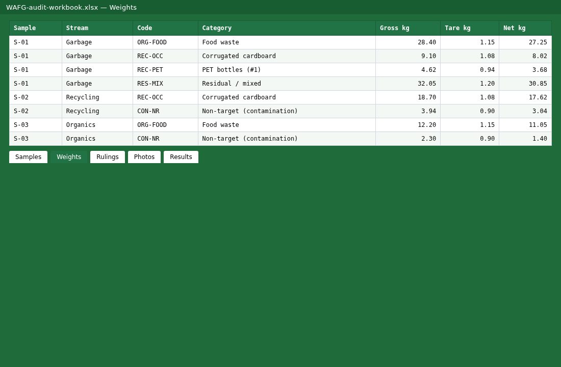
Worked-Example Workbook

The Maple Centre dataset as a downloadable workbook: the long-format Weights sheet, every calculation on this page as an inspectable formula, and the pivot that produces the dashboard export.

XLSX — blank workbook and Maple Centre worked example

Related

Sample-size and precision: the §03 calculator. Category codes and the 73-material crosswalk: §06. Dataset structure and entry checks: §08. Turning these results into program decisions: §11.